In particular, it is often difficult to observe the underlying dynamics of the learning process in neuroevolution and neural network optimization. To address this gap and open up the process to observation, we introduce Visual Inspector for Neuroevolution (VINE), an open source interactive data visualization tool aimed at helping those who are interested in neuroevolution to better understand and explore this family of algorithms. We hope this technology will inspire new innovations and applications of neuroevolution in the future.
VINE can illuminate both ES- and GA-style approaches. In this article, we focus on visualizing the result of applying ES to the Mujoco Humanoid Locomotion task as our example.
In the conventional application of ES (as popularized by OpenAI), a group of neural networks called the pseudo-offspring cloud are optimized against an objective over generations. The parameters of each individual neural network in the cloud are generated by randomly perturbing the parameters of a single “parent” neural network. Each pseudo-offspring neural network is then evaluated against the objective: in the Humanoid Locomotion Task, each pseudo-offspring neural network controls the movement of a robot, and earns a score, called its fitness, based on how well it walks. ES constructs the next parent by aggregating the parameters of pseudo-offspring based on these fitness scores (almost like a sophisticated form of multi-parent crossover, and also reminiscent of stochastic finite differences). The cycle then repeats.
 |
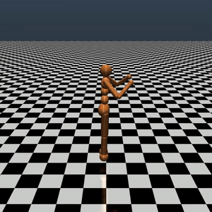 |
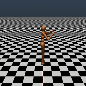
| Figure 1: Simulated robots trained to walk with genetic algorithms (left) and evolutionary strategies (right). |
Using VINE
To take advantage of VINE, behavior characterizations (BCs) for each parent and all pseudo-offspring are recorded during evaluation. Here, a BC can be any indicator of the agent’s behavior when interacting with its environment. For example, in Mujoco we simply use the agent’s final {x, y} location as the BC, as it indicates how far the agent has moved away from origin and to what location.
The visualization tool then maps parents and pseudo-offspring onto 2D planes according to their BCs. For that purpose, it invokes a graphical user interface (GUI), whose major components consists of two types of interrelated plots: one or more pseudo-offspring cloud plots (on separate 2D planes), and one fitness plot. Illustrated in Figure 2, below, a pseudo-offspring cloud plot displays the BCs for the parent and pseudo-offspring in the cloud for every generation, while a fitness plot displays the parent’s fitness score curve as a key indicator of progress over generations.
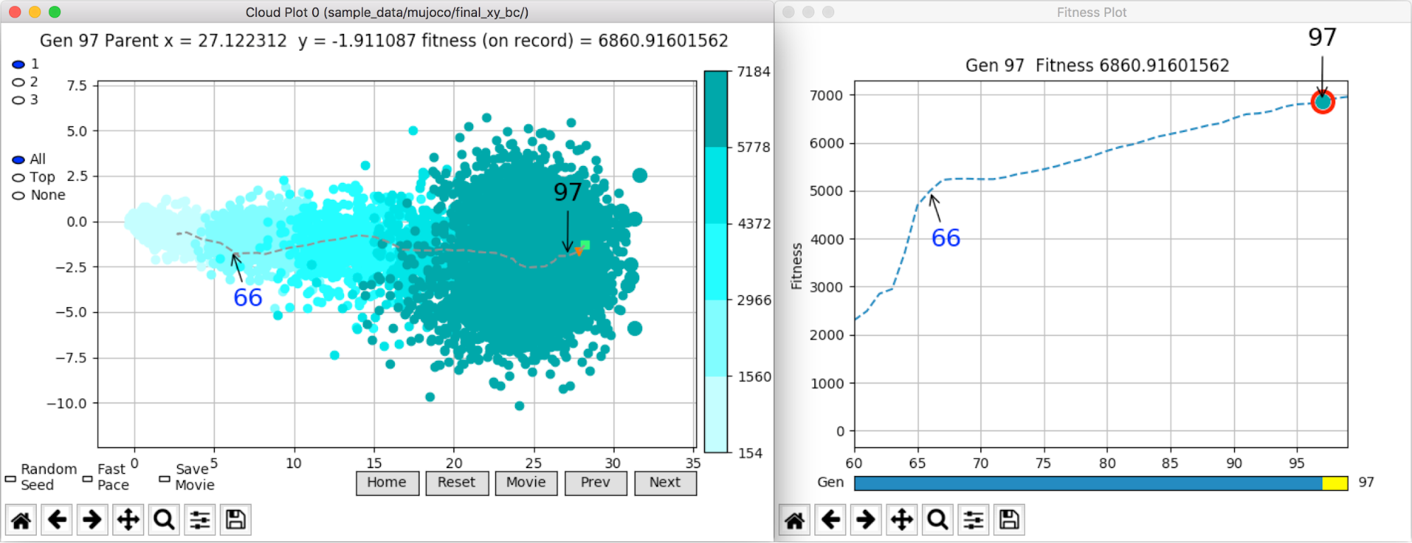
Figure 2: Examples of a pseudo-offspring cloud plot and a fitness plot.
Users then interact with these plots to explore the overall trend of the pseudo-offspring cloud as well as the individual behaviors of any parent or pseudo-offspring over the evolutionary process: (1) users can visualize parents, top performers, and/or the entire pseudo-offspring cloud of any given generation, and explore the quantitative and spatial distribution on the 2D BC plane of pseudo-offspring with different fitness scores; (2) users can compare between generations, navigate through generations to visualize how the parent and/or the pseudo-offspring cloud is moving on the 2D BC plane, and how such moves relate to the fitness score curve (as demonstrated in Figure 3, a full movie clip of the moving cloud can be generated automatically); (3) clicking on any point on the cloud plot reveals behavioral information and the fitness score of the corresponding pseudo-offspring.
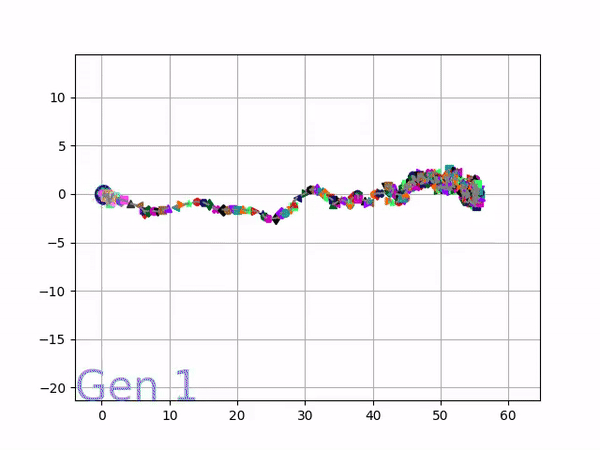
Figure 3: Visualizing the evolution of behaviors over generations. The color changes in each generation. Within a generation, the color intensity of each pseudo-offspring is based on the percentile of its fitness score in that generation (aggregated into five bins).
Additional use cases
The tool also supports advanced options and customized visualizations beyond the default features. For example, instead of just a single final {x, y} point, the BC could instead be each agent’s full trajectory (e.g., the concatenated {x, y} for 1,000 time steps). In that case, where the dimensionality of the BC is above two, dimensionality reduction techniques (such as PCA or t-SNE) are needed to reduce the dimensionality of BC data to 2D. Our tool automates these procedures.
The GUI is capable of loading multiple sets of 2D BCs (perhaps generated through different reduction techniques) and displaying them in simultaneous and connected cloud plots, as demonstrated in Figure 4. This capability provides a convenient way for users to explore different BC choices and dimensionality reduction methods. Furthermore, users can also extend the basic visualization with customized functionality. ‘Figure 4 exhibits one such customized cloud plot that can display certain types of domain-specific high-dimensional BCs (in this case, an agent’s full trajectory) together with the corresponding reduced 2D BCs. Another example of a customized cloud plot, in Figure 5, allows the user to replay the agent’s deterministic and stochastic behavior it produces when interacting with an environment.
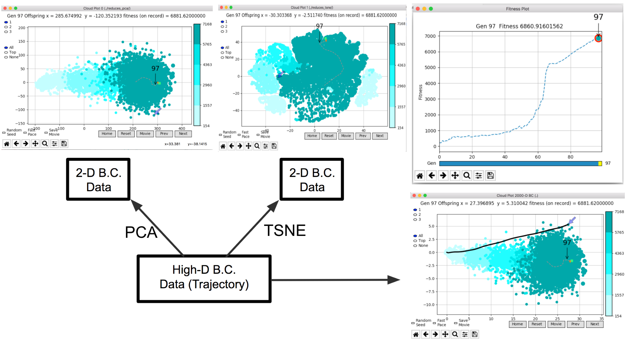
Figure 4: Visualizations of multiple 2D BCs and a high-dimensional BC along with a fitness plot.
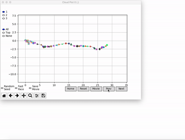
Figure 5: VINE allows users to view videos of any agent’s deterministic and stochastic behaviors.
The tool is also designed to work with domains other than locomotion tasks. Figure 6, below, demonstrates a cloud plot that visualizes ES training agents to play Frostbite, one of the Atari 2600 games, where we use the final emulator RAM state (integer-valued vectors of length 128 that capture all the state variables in a game) as the BC and apply PCA to map the BC onto a 2D plane.
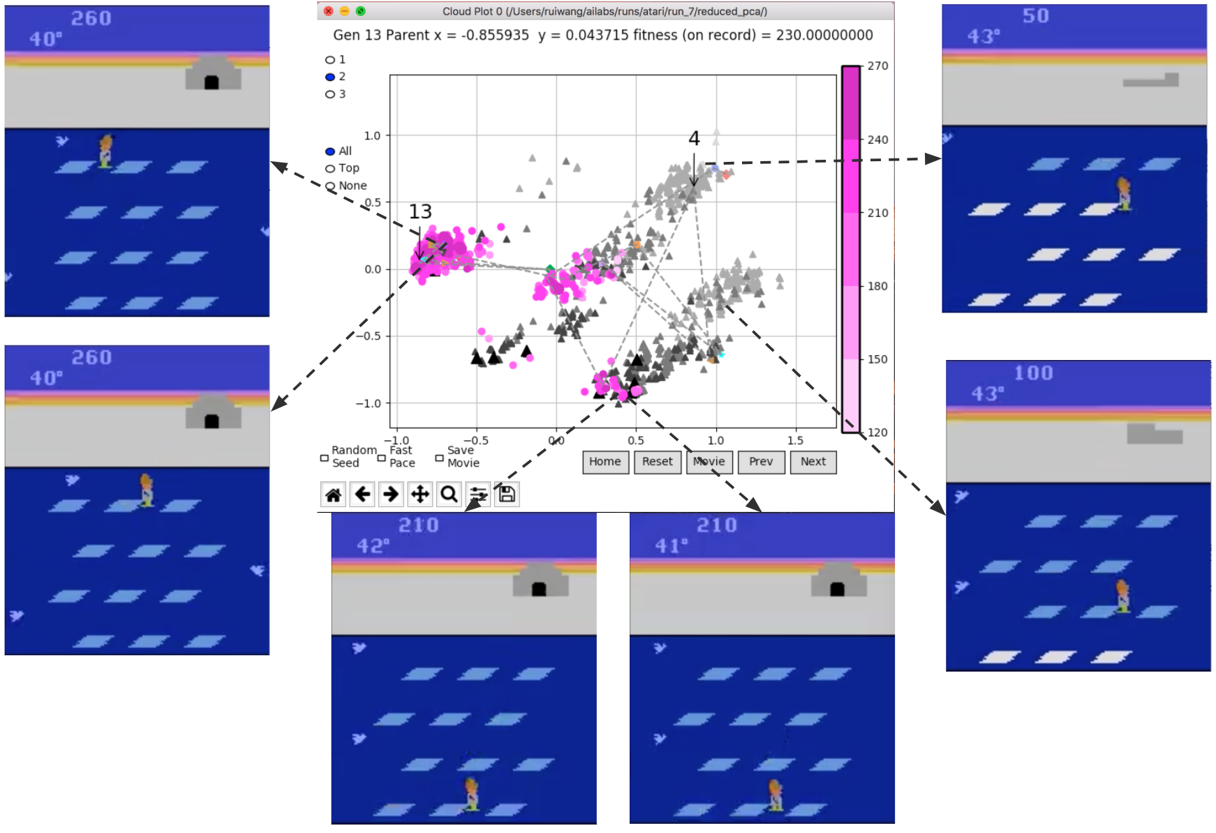
Figure 6: Visualizing agents learning to play Frostbite.
From the plot, we can observe that as evolution progresses, the pseudo-offspring cloud shifts towards the left and clusters there. The ability to see the corresponding video of each of these agents playing the game lets us infer that each cluster corresponds to semantically meaningful distinct end states.
VINE also works seamlessly with other neuroevolution algorithms such as GAs, which maintain a population of offspring over generations. In fact, the tool works independently of any specific neuroevolution algorithm. Users only need to slightly modify their neuroevolution code to save the BCs they pick for their specific problems. In the code release, we provide such modifications to our ES and GA implementations as examples.
Next steps
Because evolutionary methods operate over a set of points, they present an opportunity for new types of visualization. Having implemented a tool that provides visualizations we found useful, we wanted to share it with the machine learning community so all can benefit. As neuroevolution scales to neural networks with millions or more connections, gaining additional insight through tools like VINE is increasingly valuable and important for further progress.
VINE can be found at this link. It is lightweight, portable, and implemented in Python.
Acknowledgements
We thank Uber AI Labs, in particular Joel Lehman, Xingwen Zhang, Felipe Petroski Such, and Vashisht Madhavan for valuable suggestions and helpful discussions.